Make data connected again!
Living in a highly connected world ~ a large amount of related data is created on a daily basis. Although these relationships allow us to have valuable insights into how various data points (actions, people etc.) are associated with each other, affect each other, or may influence each other in the future, they often get lost once the data is stored in common relational tables or other general NoSQL data stores.

Fig. 1: Illustration of the connected web of data
The graph data model (like shown in Figure 2) faces the problem of “isolated data points” by addressing relationships as first class citizens. As an example, a user’s post/tweet and its additional information (hashtags, links, sources etc.) can be expressed as a graph and analyzed to understand how the post influenced the user’s follower base.
This is just a simple example of showing that graphs are very well suited for finding patterns and anomalies among large and complex data volumes.
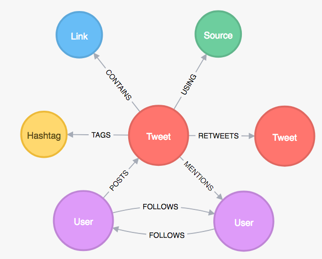
Fig. 2: Social media graph
When first starting off working with graphs and graph databases, one notices that the graph data model and its corresponding query language differ from one data store to another. Often graphs are expressed as property graphs (Figure 3).
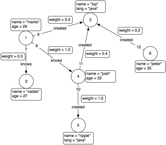
Fig. 3: Property graph model
The property graph consists of triples, which are two nodes that are connected with each other through a directed edge. Each node has its own unique ID, and may have several properties that expose more detailed information about it (e.g. name=’’vadas’’). Each edge expresses the relationship between two nodes, has an unique ID, and can also have multiple properties. The data model of a graph can vary from one company to another companies context. So does the underlying graph storage engine, varying from key-value- to document-oriented-, native graph data stores & many more. Some of them keep the graph data in-memory (for fast operations before storing it on-disk), while others store the data on a secondary storage level right away, making use of smart storage data structures like LSM- or B+ trees that provide an indexed access to the data which reduces the number of disk accesses (slow access) when operations are performed on the data.
BUT, it doesn’t take one a lot of time to encounter the weakpoint of this variety of graph models & databases: Data Integration. Different companies often use their own derivation of a property graph model (different datatypes, structure of properties, IDs etc.), making it almost impossible to integrate the data from one company’s context to another.
To tackle this problem: Tim-Berners Lee, the inventor of the World Wide Web, introduced his vision of his so called Next Web, or Linked Open Data (good introduction video). The Next Web’s underlying technology is considered to be available as Open Source and to be based on 4 rules, that Mr. Berners-Lee proposed:
- Use URIs as names for things
- Use HTTP URIs so that people can look up those names.
- When someone looks up a URI, provide useful information, using the standards (RDF, SPARQL)
- Include links to other URIs, so that they can discover more things.
RDF or Resource Description Framework provides a graph model (Figure 4) that consists of triples (2 nodes), the subject + object node and an edge or predicate that represents a directed connection from subject to object. So far nothing new compared to the property graph model, but the power of RDF’s graph model is that each element(subject, predicate, object) is represented solely by one URI(each object may be represented by values of different data types aswell). In addition to this RDF’s full potential blossoms out when the graph is build using common vocabularies such as rdfs, a W3C-recommended vocabulary (for more info, see RDFS). It’s this uniqueness and detailed structure that make RDF so powerful, enabling easy data integration across multiple collaborating units. The language to query an RDF-graph is called SPARQL. SPARQL is a declarative query language (user decides beforehand what data to retrieve) that expresses graph pattern queries across diverse data sources, whether the data is stored natively as RDF or viewed as RDF via middleware. Many industries like the genomic engineering industry adapted RDF, because they deal with large, complex, highly connected datasets + strongly rely on a consistent “uniform” of the graph data representation that is used by many different genomic companies and labs.
Fig. 4: RDF Graph Model
As applications become more complex in terms of their size (Big Data), comprising data from a variety of devices, platforms, sensors etc., the number of industries that adopt RDF and contribute to advance it’s technology is steady growing. Although there are many different graph databases out there (popular one: Neo4j) most of them store their data expressed in the property graph model. Only a few support RDF and those who do don’t scale-out (Big Data requirement) very well. As in Intern at Koneksys, located in San Francisco,CA, I created a tool that compiles an RDF graph to a Apache Spark GraphFrame and runs SPARQL queries on it. GraphFrames’ ability to run graph queries and graph Algorithms(e.g. PageRank) in-memory (fast access) & to fetch data from a variety of sources make it a great tool for RDF applications that work with large datasets. In addition to this GraphFrames’ internal query language has a common denominator with SPARQL which is it’s capability for querying graph patterns. It’s an Apache Spark compatible package that was introduced by the AMPLab at UC Berkeley and is actively being developed (for more info, see GraphFrames). Due to it’s promising technology it is considered to be added to Apache Spark’s ecosystem soon, which will make it part of a large and active user-community. A GraphFrame is based on two DataFrames, the data model of Spark SQL, one for the nodes (internal name: vertices) and one for the edges. Querying a GraphFrame will output another DataFrame that itself can be used to create a new GraphFrame. A DataFrame and therefore GraphFrame can be created using a large variety of data sources like Apache Cassandra, HBase, Neo4j, HDFS and many more. Basically every database can be used as an input source if a fitting Connector is created beforehand. This tool is currently being tested in a cluster (HDFS-cluster) and may also be tested in a single node setup, using various dataset sizes corresponding to the rules defined by The Berlin SPARQL Benchmark (BSBM) that compares the performance of RDF applications. Feel free to test the tool and read the documentation about it’s architecture on GitHub: SPARQL2GF.